Rerun 0.16 gives you more blueprint control from code
Our 0.16 release introduced Blueprint APIs that let you define your layout and content from code. This release is exposing view properties in the blueprint! With that you’re able to stylize your visualizations from code. Included in this release is a first set of view properties, there will be many more in future releases. In addition, this release comes with significant changes in infrastructure, particularly we’re deprecating the concept of timeless data and are introducing static data.
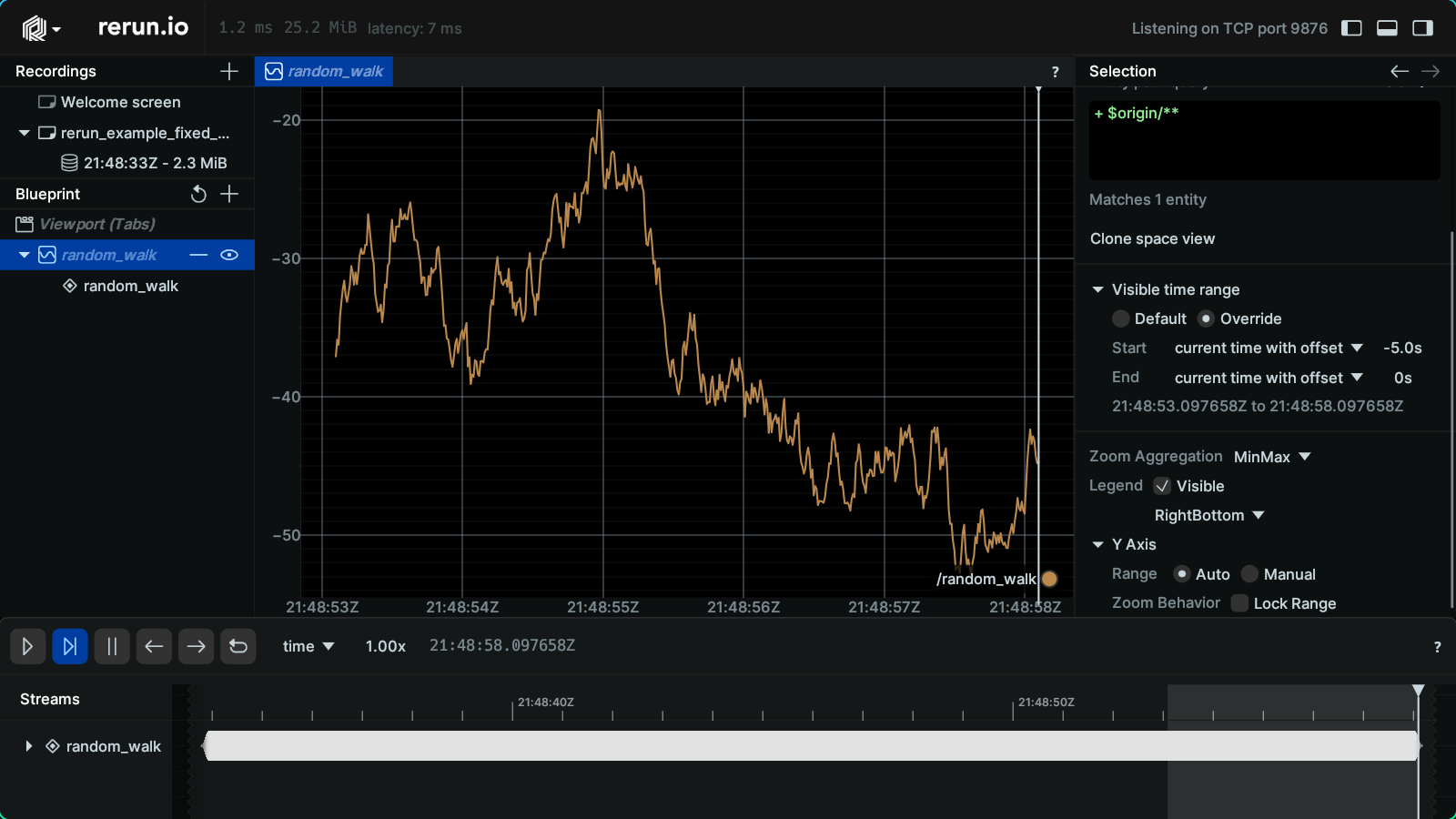
An example of view properties you can define from code is visible time range. Say you are live-streaming IMU data over a longer time period. Instead of accumulating all of that data in the view you can now define a relative time window.
Define visible time range define-visible-time-range
To create a trailing 5 second window plot, you can specify your TimeSeriesView like this:
rrb.TimeSeriesView(
    origin="plot_path",
    time_ranges=rrb.VisibleTimeRange(
        timeline="time",
        start=rrb.TimeRangeBoundary.cursor_relative(seconds=-5.0),
        end=rrb.TimeRangeBoundary.cursor_relative(),
    )
)
That will give you a plot showing you the last 5 seconds of your in streaming data. You will see a highlight on your timeline to indicate the data range currently shown. If you want to dive deeper check out the tutorial on how to create a fixed window plot.

Stylize your visualization stylize-your-visualization
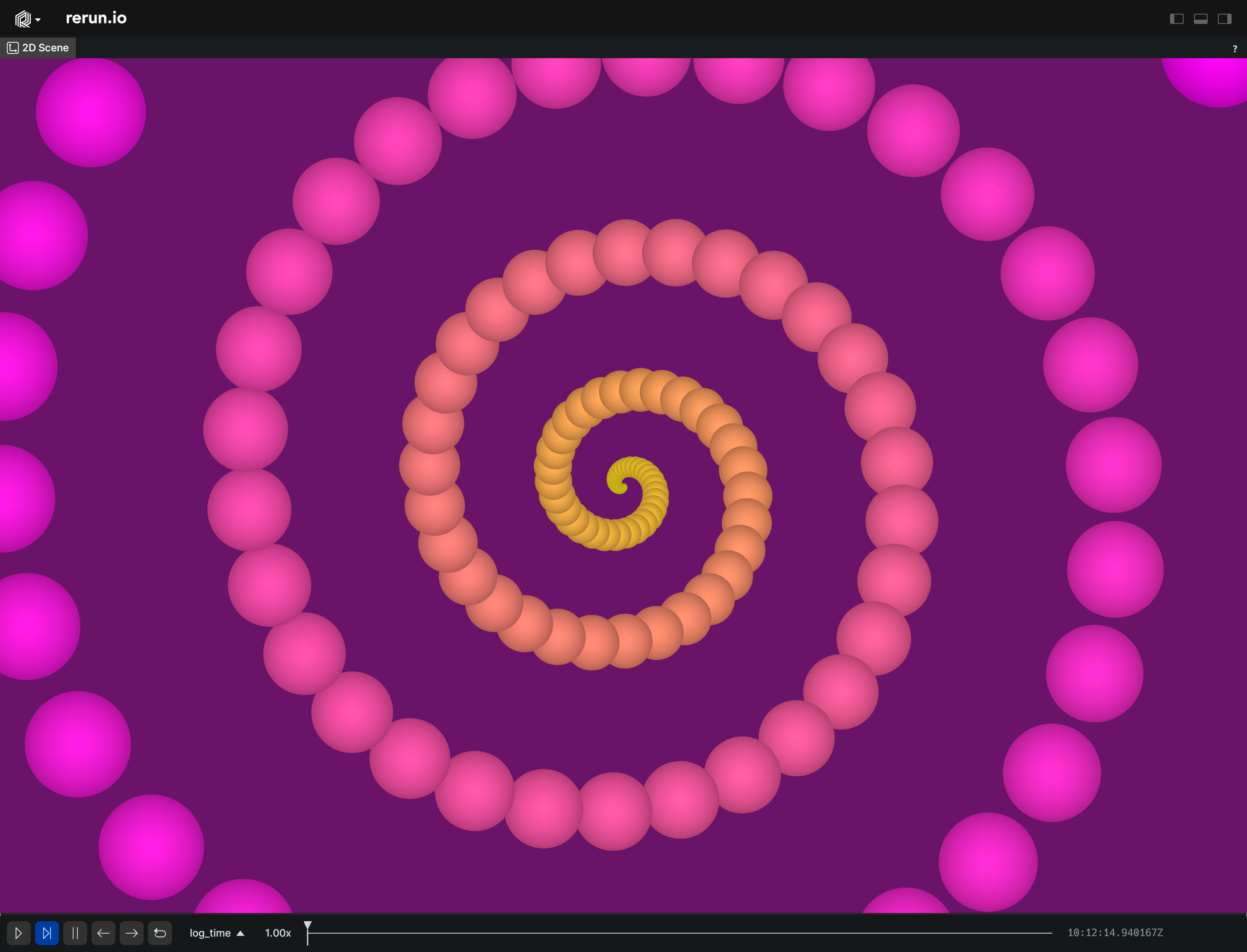
Other view properties included in this release are background color for 2D and 3D views, and visual bounds for 2D views. The code snippet is showing how to create a spiral of points, and then setup a 2D view, name it, define the background color, define visual bounds, and collapse all side panels through a blueprint.
"""Use a blueprint to customize a Spatial2DView."""

import numpy as np
import rerun as rr
import rerun.blueprint as rrb

rr.init("rerun_example_spatial_2d", spawn=True)

# Create a spiral of points:
n = 150
angle = np.linspace(0, 10 * np.pi, n)
spiral_radius = np.linspace(0.0, 3.0, n) ** 2
positions = np.column_stack((np.cos(angle) * spiral_radius, np.sin(angle) * spiral_radius))
colors = np.dstack((np.linspace(255, 255, n), np.linspace(255, 0, n), np.linspace(0, 255, n)))[0].astype(int)
radii = np.linspace(0.01, 0.7, n)

rr.log("points", rr.Points2D(positions, colors=colors, radii=radii))

# Create a Spatial2D view to display the points.
blueprint = rrb.Blueprint(
    rrb.Spatial2DView(
        origin="/",
        name="2D Scene",
        # Set the background color
        background=[105, 20, 105],
        # Note that this range is smaller than the range of the points,
        # so some points will not be visible.
        visual_bounds=rrb.VisualBounds2D(x_range=[-5, 5], y_range=[-5, 5]),
    ),
    collapse_panels=True,
)

rr.send_blueprint(blueprint)
The resulting visualization looks like this:

If you want to learn more check out our new small examples for each view showing all available options in our docs. We will continue to add new options over the upcoming releases.
Timeless data replaced by static data timeless-data-replaced-by-static-data
With 0.16 we are deprecating the concept of timeless data and are introducing static data. Except for the name change, they behave similarly in most use cases.
Static data is data that shows up at all times, on all timelines. If you have been using timeless data, check out the migration guide.
🤗 Huggingface’s Gradio API and Rerun -huggingfaces-gradio-api-and-rerun
And lastly, we have been experimenting with how to make Rerun useful on Huggingface Spaces. You can find an example of that here. Included in this release is further ground work to make the Rerun Gradio integration more performant. Most things for this already landed in this release and we'll soon build more direct support on top.
If you run into any problems open an issue on Github or talk to us on Discord. If you’re showing your visualizations on social please tag us ❤️ And please leave us a star on Github, that really helps increasing visibility of the project ⭐️
As always, we hope you enjoy Rerun!